FreeSeed review FreeSeed review

2026.08.12 paper-review

Ma et al., FreeSeed: Frequency-band-aware and Self-guided Network for Sparse-view CT Reconstruction, MICCAI 2023

The paper is two pieces: FreeNet and SeedNet. FreeNet bakes the physics of the problem into the architecture, and SeedNet implements a loss function in the shape of a network(?).

1. What sparse-view CT is

CT fires X-rays from many angles and inverts the projection data into a cross-sectional image. More angles mean more radiation dose for the patient, so sparse-view CT cuts the dose by using fewer angles.

Fewer angles mean less dose and faster scans. The catch: feed that thin data into FBP, the standard reconstruction algorithm, and you get streak artifacts running across the whole image. Bad enough to interfere with diagnosis.

Notation first:

symbol	what it is
$I_s$	sparse-view image, streaked (input)
$I_f$	full-view image, clean (ground truth)
$A$	artifact, $A = I_s - I_f$
$N_v$	number of views (18, 36, 72, 144)

The paper goes after two problems.

The artifact spreads across the entire image, so a local CNN struggles to catch it
The loss treats every pixel the same, so the output smears into blur

FreeNet handles the first, SeedNet the second.

2. FreeNet

2.1 Predict the artifact, not the clean image

FreeNet doesn’t produce the restored image directly. It predicts the artifact and subtracts it.

\hat A = \Theta(I_s), \qquad \hat I = I_s - \hat A

\mathcal{L}_{art} = \lVert A - \hat A \rVert^2

Since $I_f - \hat I = \hat A - A$ , we end up with $\mathcal{L}_{art} = \lVert I_f - \hat I\rVert^2$ . The loss value is identical to predicting the restored image directly. The point of targeting the artifact is that the answer the model has to learn gets easier. Mathematically equivalent choices can still train differently.

Drawing a clean CT means knowing bones, organs, and soft tissue, all of it. The artifact is one streak pattern caused by sparse angles, and it barely changes from patient to patient
It also unlocks the frequency trick below

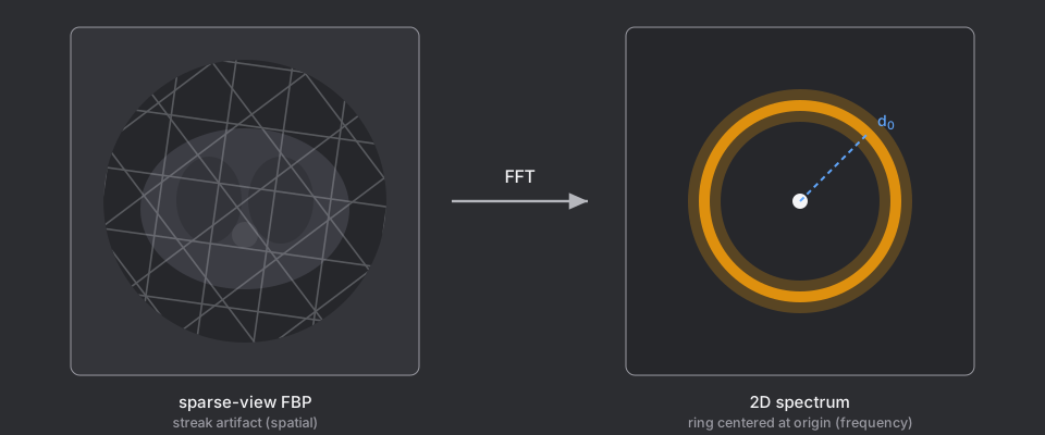
2.2 In frequency space, the artifact is a ring

The paper folds its observation about the artifact into the architecture, so the model can learn it indirectly. Fourier-transform the streaks and you get a ring centered at the origin.

Streak artifact (spatial domain) becomes a ring centered at the origin (frequency domain) under the Fourier transform

2.3 FFC

The new idea: FFC (Fast Fourier Convolution). Split the channels in half. One half goes through a regular CNN; the other half gets Fourier-transformed first, then convolved.

A conv in the frequency domain has a receptive field spanning the whole image, which makes the artifact easier to learn.

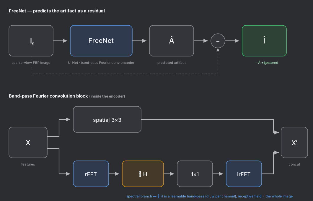
FreeNet architecture: a U-Net predicting the artifact as a residual. Each encoder block splits channels in half into spatial/spectral branches

Two extra parameters on top.

Z_{in} = \mathcal{F}_{real}\{X_{in}\}, \quad Z_{out} = f(Z_{in} \odot H), \quad X_{out} = \mathcal{F}_{real}{}^{-1}\{Z_{out}\}

H = \exp\left[-\left(\frac{D^2 - d_0{}^{2}}{wD + \epsilon}\right)^2\right]

$D$ is the distance map from the origin, and the bandwidth $w$ and radius $d_0$ are learnable parameters. Each channel gets its own pair.

The paper doesn’t hand the model “the artifact lives in this band” as an answer. It lays down a structure where the model can use that knowledge.

3. SeedNet

3.1 This is a loss, not an architecture

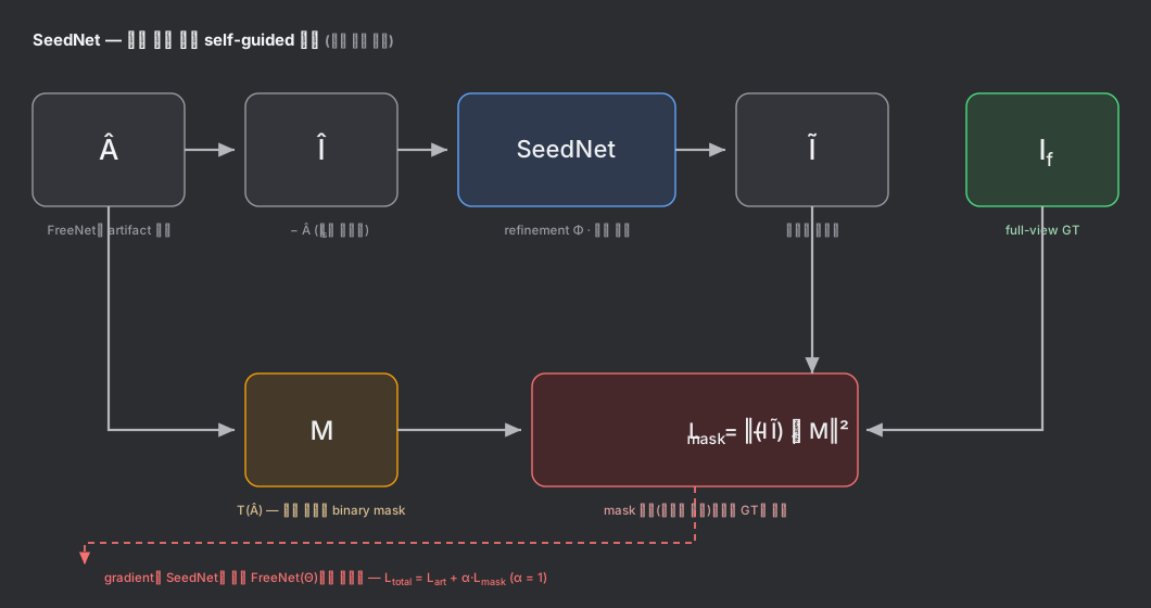
The easiest place to get confused. SeedNet is not a second restoration stage. It’s attached only during training and thrown away afterwards. Inference is FreeNet alone, and the cost doesn’t grow.

\tilde I = \Phi(\hat I)

M = \mathcal{T}(\hat A) \quad (\hat A \text{ binarized with its mean as the threshold})

\mathcal{L}_{mask} = \lVert (I_f - \tilde I)\odot M \rVert^2

The residual holds $\tilde I$ , not $\hat I$ . FreeNet’s output isn’t graded directly; it gets passed through once more, and that result is what’s graded.

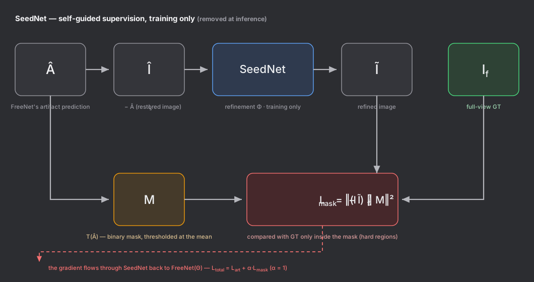
SeedNet architecture: build a mask from the predicted artifact, then compare SeedNet's refined output against GT only inside the mask region

\mathcal{L}_{total} = \mathcal{L}_{art} + \alpha \mathcal{L}_{mask} \qquad (\alpha = 1)

SeedNet → $\mathcal{L}_{mask}$ only
FreeNet → $\mathcal{L}_{total}$
$\mathcal{L}_{mask}$ is shared by both. For FreeNet, the gradient arrives through SeedNet

3.2 The obvious approach fails

Given a mask, the first thing anyone thinks of is extra loss weighting.

\mathcal{L}_{1+mask} = \lVert (A - \hat A)\odot(1+M)\rVert^2

“Double the weight where the artifact is bad.” It fails.

Routed through SeedNet instead, the gradient passes through $\Phi$ and spreads out spatially. The staircase at the mask boundary gets smoothed away.

3.3 Training order

Five steps per batch.

1. Î, Â = Θ(Is)        FreeNet forward
2. Ĩ  = Φ(Î)           SeedNet forward
3. update Φ only, with L_mask  → Φ'
4. Ĩ' = Φ'(Î)          forward again through the updated Φ
5. update Θ with L_total

FreeNet gets graded by the SeedNet that just improved. Without step 4, FreeNet never hears SeedNet’s demand to pull out more of the recoverable information.

4. Why does it beat MSE at PSNR? A guess

$\text{PSNR} = 10\log_{10}(\text{MAX}^2/\text{MSE})$ , so lowering MSE and raising PSNR are the same statement. Then why does mixing in something else beat the loss aimed straight at the metric?

A loss function does two jobs.

Define what counts as good
Supply usable gradients throughout training

MSE is perfect at the first job. At the second it’s mediocre. Same reason classification trains on cross-entropy while the metric is accuracy.

Blur as a refuge

The MSE optimum is the conditional mean. What the network actually reaches, though, is the conditional mean given the features it currently extracts.

The problem: looking at the output, the two cases are indistinguishable.

Blurry because the input genuinely lacks the information
Blurry because the information is there and the network fails to extract it

MSE can’t tell these apart. So smearing in low-confidence regions can be a winning move.

$\Phi$ can tell them apart. If the information survives, it revives it; if it’s gone, nothing comes back. That changes the question $\mathcal{L}_{mask}$ asks.

MSE asks “how wrong is it.” $\mathcal{L}_{mask}$ asks “is it wrong in a fixable way.”

Blur stops being an equilibrium, so FreeNet learns to actually dig more information out of $I_s$ , and the answer itself moves closer to the ground truth. Even at inference, with $\Phi$ gone.

This whole section is my reconstruction; it’s not in the paper. The paper’s own explanation is the discontinuous-gradient point in 3.2.

What this interpretation predicts

Under conditions where the information is physically absent, SeedNet should hurt. Blur is the right answer there, and SeedNet demands the impossible.

$N_v=18$ is that condition, and performance does drop.

$N_v$	18	36	72	144
baseline	35.04	37.63	41.95	45.96
baseline + SeedNet	34.49	38.35	42.89	48.64
delta	−0.55	+0.72	+0.94	+2.68

5. Wrap-up

FreeNet: a module that reflects the character of the noise this problem actually produces
SeedNet: my read is they wanted a perceptual loss and couldn’t use one, since ImageNet features don’t transfer to this domain. Using SeedNet to block the main model from settling on blurry answers, indirectly asking it to dig out more information instead: that part is genuinely clever. First structure of this kind I’ve seen. Does it only work on structural noise? Only in domains where a perceptual loss is hard to use? Either way, a new module worth applying somewhere.

Ma et al., FreeSeed: Frequency-band-aware and Self-guided Network for Sparse-view CT Reconstruction, MICCAI 2023

FreeNet과 SeedNet 두 개로 되어 있다. FreeNet은 문제의 물리적 성질을 아키텍처에 심었고, SeedNet은 손실 함수를 아키텍처 형태로 구현(?)했다.

1. Sparse-view CT가 뭔가

CT는 X선을 여러 각도에서 쏘고, 그렇게 얻은 투영 데이터를 역변환해서 단면 영상을 만든다. 여러 각도로 사진을 많이 찍을수록 환자의 피폭량도 늘어나는데, 피폭량을 줄이기 위해 촬영 각도를 덜 쓰는 것이 sparse-view CT다.

각도를 줄이면 피폭도 줄고 촬영도 빨라진다. 대신 재구성 알고리즘인 FBP에 적은 데이터를 넣으면 영상 전체를 가로지르는 줄무늬 아티팩트가 생긴다. 진단을 방해할 만큼 심하다.

기호부터 정리하면:

기호	뭔지
$I_s$	sparse-view 영상, 줄무늬 있음 (입력)
$I_f$	full-view 영상, 깨끗함 (정답)
$A$	아티팩트, $A = I_s - I_f$
$N_v$	각도 수 (18, 36, 72, 144)

논문이 잡으려는 문제는 두 개다.

아티팩트가 영상 전체에 퍼져 있어서 국소적인 CNN으로는 잡기 어렵다
손실이 모든 픽셀을 똑같이 취급해서, 결과가 뿌옇게 뭉개진다

FreeNet이 1번, SeedNet이 2번 담당이다.

2. FreeNet

2.1 깨끗한 영상 말고 아티팩트를 예측한다

FreeNet은 복원 영상을 바로 만들지 않는다. 아티팩트를 예측하고 그걸 뺀다.

\hat A = \Theta(I_s), \qquad \hat I = I_s - \hat A

\mathcal{L}_{art} = \lVert A - \hat A \rVert^2

$I_f - \hat I = \hat A - A$ 니까, 결국 $\mathcal{L}_{art} = \lVert I_f - \hat I\rVert^2$ 다. 손실값 자체는 복원 영상을 직접 예측하는 거랑 똑같다. 굳이 아티팩트를 타깃으로 한 이유는 모델이 알아야 할 정답이 쉬워지기 때문이다. 수학적으로 동일해도 학습에 영향을 준다.

깨끗한 CT를 그리려면 뼈, 장기, 연조직의 특징을 전부 알아야 함. 아티팩트는 각도가 성겨서 생기는 줄무늬 패턴 하나만 알면 된다. 환자가 바뀌어도 거의 같다
그리고 아래 나올 주파수 트릭을 쓸 수 있다

2.2 아티팩트를 주파수 공간에서 보면 링이다

논문이 관찰한 아티팩트의 특징을 모델이 간접적으로 더 잘 학습할 수 있도록 아키텍처에 반영한다. 줄무늬 아티팩트를 푸리에 변환하면 원점 중심의 링 모양이 생긴다.

줄무늬 아티팩트(공간 영역)를 푸리에 변환하면 원점 중심의 링(주파수 영역)이 된다

2.3 FFC

새 아이디어 FFC(Fast Fourier Convolution). 채널을 반으로 나눠서 한쪽은 일반 CNN, 다른 쪽은 푸리에 변환 후 CNN한다.

주파수 영역에서 conv를 하면 receptive field가 전역에 걸쳐서 모델이 아티팩트를 배우기 쉬워짐.

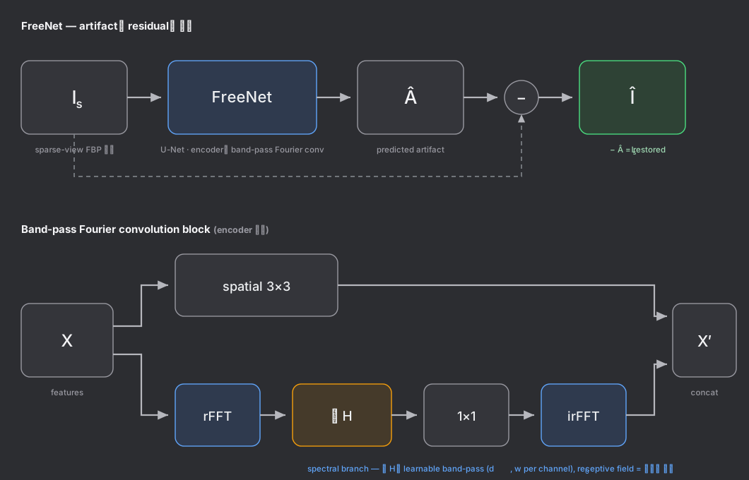
FreeNet 구조 — U-Net으로 artifact를 residual 예측. encoder 블록은 채널을 반씩 나눠 spatial/spectral branch로 처리한다

여기에 파라미터 두 개 추가.

Z_{in} = \mathcal{F}_{real}\{X_{in}\}, \quad Z_{out} = f(Z_{in} \odot H), \quad X_{out} = \mathcal{F}_{real}{}^{-1}\{Z_{out}\}

H = \exp\left[-\left(\frac{D^2 - d_0{}^{2}}{wD + \epsilon}\right)^2\right]

$D$ 는 원점에서의 거리 맵이고, 대역폭 $w$ 랑 반지름 $d_0$ 이 학습 파라미터. 채널마다 한 쌍씩 따로 둔다.

“아티팩트는 이 대역에 있어” 를 정답으로 알려주는 게 아니라, 모델이 그 지식을 쓸 수 있는 구조를 깔아주는 것.

3. SeedNet

3.1 이건 아키텍처가 아니라 손실이다

제일 헷갈리기 쉬운 부분. SeedNet은 복원의 2단계가 아니다. 학습할 때만 붙어 있고 끝나면 버린다. 추론은 FreeNet 혼자 하고 비용이 안 늘어난다.

\tilde I = \Phi(\hat I)

M = \mathcal{T}(\hat A) \quad (\hat A \text{ 평균값을 임계값으로 이진화})

\mathcal{L}_{mask} = \lVert (I_f - \tilde I)\odot M \rVert^2

잔차 안에 있는 건 $\hat I$ 가 아니라 $\tilde I$ . FreeNet 출력을 바로 채점하는 게 아니라, 한 번 더 통과시킨 걸 채점함.

SeedNet 구조 — 예측된 artifact에서 mask를 만들고, SeedNet이 다듬은 결과를 mask 영역에서만 GT와 비교한다

\mathcal{L}_{total} = \mathcal{L}_{art} + \alpha \mathcal{L}_{mask} \qquad (\alpha = 1)

SeedNet → $\mathcal{L}_{mask}$ 만
FreeNet → $\mathcal{L}_{total}$
$\mathcal{L}_{mask}$ 는 둘이 같이 씀. FreeNet한테는 SeedNet을 거쳐서 그래디언트가 온다

3.2 직관적인 방법의 실패

마스크가 있으면 제일 먼저 떠오르는 건 손실에 추가 가중치를 주는 방법.

\mathcal{L}_{1+mask} = \lVert (A - \hat A)\odot(1+M)\rVert^2

“아티팩트 심한 데 가중치 두 배” — 실패.

SeedNet을 거치면 그래디언트가 $\Phi$ 를 통과하면서 공간적으로 번진다. 마스크 경계의 계단이 뭉개지는 것.

3.3 학습 순서

배치마다 이 다섯 개가 돈다.

1. Î, Â = Θ(Is)        FreeNet 순전파
2. Ĩ  = Φ(Î)           SeedNet 순전파
3. L_mask 로 Φ만 갱신   → Φ'
4. Ĩ' = Φ'(Î)          갱신된 Φ로 다시 순전파
5. L_total 로 Θ 갱신

FreeNet은 방금 개선된 SeedNet한테 채점받는다. 4번이 없으면 seednet의 복원 가능한 정보를 더 가져오라는 요구를 freenet이 알지 못함.

4. 왜 MSE보다 PSNR이 잘 나올까? 추측

$\text{PSNR} = 10\log_{10}(\text{MAX}^2/\text{MSE})$ , MSE 낮추기랑 PSNR 올리기는 같은 말인데, 지표를 직접 겨냥한 것보다 딴 걸 섞은 게 왜 지표에서 이기지?

손실 함수는 두 가지 일을 한다.

뭐가 좋은지 정의
학습 내내 쓸 만한 그래디언트 공급

MSE는 1번에서 완벽. 2번에서는 별로다. classification에서 정확도가 지표인데 cross-entropy로 학습하는 거랑 같다.

흐릿한 도피처

MSE 최적해는 조건부 평균이다. 근데 네트워크가 실제로 도달하는 건 지금 뽑아낸 특징에 대한 조건부 평균이다.

문제는 출력에서 보면 두 경우가 똑같아 보인다는 것.

입력에 정보가 진짜 없어서 흐린 것
정보는 있는데 네트워크가 못 꺼내서 흐린 것

MSE는 이 둘을 구분 못 한다. 그래서 자신 없는 영역에서 뭉개는 게 이득이 될 수도 있다.

$\Phi$ 는 이 둘을 구분함. 정보가 남아 있으면 되살리고 없으면 못 되살리니까. 그래서 $\mathcal{L}_{mask}$ 가 던지는 질문이 바뀐다.

MSE는 “얼마나 틀렸나”, $\mathcal{L}_{mask}$ 는 “고칠 수 있게 틀렸나”

뭉개는 게 더 이상 균형점이 아니니까, FreeNet은 $I_s$ 에서 정보를 실제로 더 꺼내는 쪽으로 학습되며 답 자체가 정답에 가까워진다. $\Phi$ 가 없는 추론 때도.

이 절 전체가 논문에 없는 내 재구성이다. 논문 설명은 3.2의 불연속 그래디언트 하나.

이 해석이 맞으면 예측되는 것

정보가 물리적으로 없는 조건에서는 SeedNet이 해로워야 한다. 흐린 게 정답인데 불가능한 요구를 하기 때문이다.

$N_v=18$ 이 그 조건이고, 실제로 성능이 낮아진다.

$N_v$	18	36	72	144
baseline	35.04	37.63	41.95	45.96
baseline + SeedNet	34.49	38.35	42.89	48.64
차이	−0.55	+0.72	+0.94	+2.68

5. 정리

FreeNet: 생기는 노이즈 특성을 잘 반영한 모듈 도입
SeedNet: perceptual loss를 못 써서 쓴 듯 — ImageNet과 도메인 특성이 달라서 사용 못 하니까. SeedNet으로 메인 모델이 블러 답을 못 내게 하고 정보를 더 파내게끔 간접 질문한 게 신박하다. 이런 구조는 처음인데 구조적인 노이즈에만 유효한 방법인가? perceptual loss를 사용하기 힘든 영역에서만 유효할까? 적용할만한 새 모듈 발견.